Colouring Noise

I’ve been characterising a high performance gyroscope at work recently by measuring the Allan variance of its rate output. From the Allan variance plot, it’s possible to visualise and calculate the various sources of noise that cause error, including quantisation noise, angular random walk, bias instability and rate random walk. Each of these noise sources is caused by a different physical process and can be differentiated by its colour. What is noise colour, you ask?

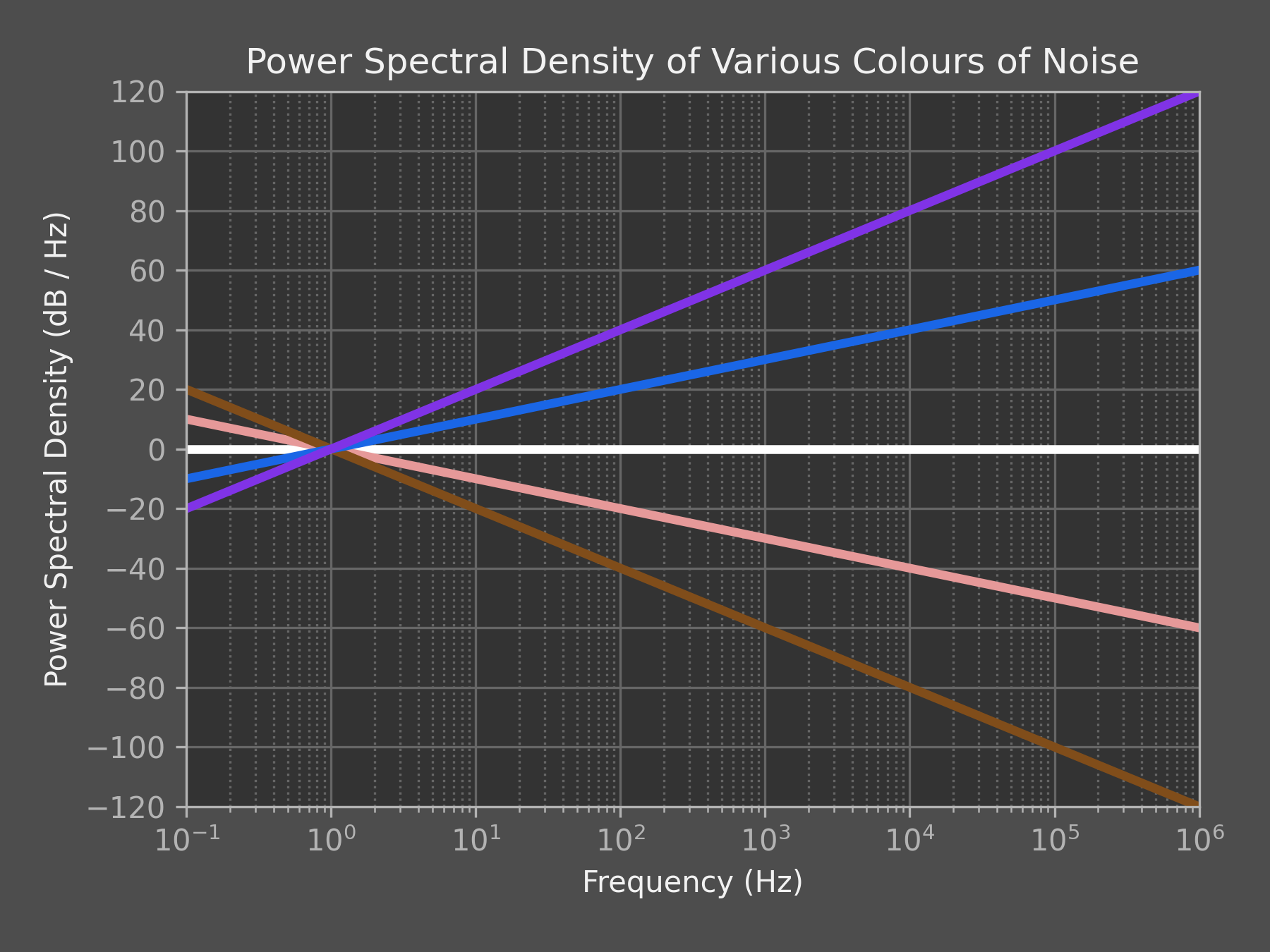
The colour of noise refers to the shape of its power spectral density (PSD). Over time, people have assigned colours to particular shapes in the power spectrum.

• White: Probably the most commonly known noise colour, it has a constant PSD for all frequencies. Background “static” in unused portions of the radio spectrum approximates white noise. In audio form, it can help block out background noise or alleviate the symptoms of tinnitus.
• Pink: Has a PSD proportional to $1/f$. This means in logarithmic space it falls off at a rate of 10 dB/decade. It shows up in many electronic components as flicker noise, and is often used by audio technicians to characterise speakers.
• Brownian: Sometimes called “brown” or “red” noise, it has a PSD proportional to $1/f^2$. Physical processes that involve a random walk generate noise with this PSD shape.
• Blue: Noise with a PSD that increases proportionally with $f$. The photons emitted due to Cherenkov radiation have this PSD. Two dimensional blue noise is commonly used in computer graphics as a pattern to nicely dither images.
• Violet: Has a PSD proportional to $f^2$. Acoustic noise in water due to tiny changes in pressure from thermal effects is best characterised by this noise colour.

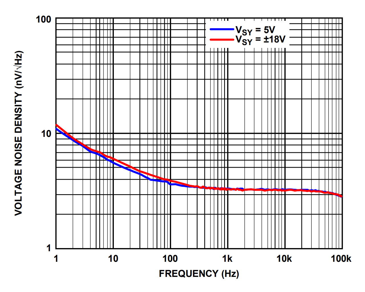
Ultimately, these colours of noise are often approximations of what we observe over specific frequency bands, and the full PSD of a process can contain multiple colours of noise mixed together. For example, the input referred voltage noise density (which is proportional to the square root of the PSD) of a typical opamp is shown below. This noise could be described as pink noise to around 200–300 Hz, and white noise up to around 50 kHz, but the final measured noise density is more complex.

Generating Coloured Noise Samples

The process of generating coloured noise is relatively simple:

1. Start with a representation of white noise signal in the frequency domain
2. Shape the signal in the frequency domain according to the PSD you’d like to achieve
3. Take the inverse Fourier transform of the shaped signal

We’ll take a look at how we can easily do this in Python using numpy, scipy and matplotlib.

Base Noise

To begin, we need to generate some white noise in the frequency domain. Ideally this noise will be normalised to have a one-sided PSD of 1.0 at all frequencies which will simplify the shaping process in the next step.

There are couple of ways to do this, with the simplest being to generate the noise in the time domain and take a Fast Fourier Transform (FFT). The PSD of uniformly sampled discrete white noise is equal to $2 \sigma ^ 2 \Delta t$, where $\sigma ^ 2$ is the variance of the noise, and $\Delta t$ is the sampling period. Let’s quickly stub out a class using this knowledge to generate our base noise.

import numpy as np


class NoiseGenerator:
    rng = np.random.default_rng()

    def generate(self, dt, n, colour=None):
        """Generates uniformly sampled noise of a particular colour.

        Parameters
        ----------
        dt : float
            Sampling period, in seconds.
        n : int
            Number of samples to generate.
        colour : function, optional
            Colouring function that specifies the PSD at a given frequency. If
            not specified, the noise returned will be white Gaussian noise with
            a PSD of 1.0 across the entire frequency range.
        
        Returns
        -------
        numpy.array
            Array of sampled noise, length `n`.
        """

        if colour:
            raise NotImplementedError("We're not ready yet!")
        
        f, x_f = self._base_noise(dt, n)

        return np.fft.irfft(x_f)

    def _base_noise(self, dt, n):
        """Produces a frequency domain representation of uniformly sampled
        Gaussian white noise.
        """
        
        # Generate Gaussian white noise in the time domain
        sigma = 1 / np.sqrt(2.0 * dt)
        x_t = rng.normal(0.0, sigma, n)

        # Calculate the frequency bins and associated FFT
        f = np.fft.rfftfreq(n, dt)
        x_f = np.fft.rfft(x)

        return f, x_f

It’s worthwhile checking here to make sure our generated noise has a constant PSD of 1.0. Welch’s method¹ is a common technique to estimate the PSD of a time domain signal. Let’s run some code to calculate a PSD estimate and plot it along with the noise signal.

import scipy.signal
import matplotlib.pyplot as plt


def plot_psd(x_t, dt, **kwargs):
    """Plots a signal and its PSD given samples and sampling period."""

    t = np.linspace(0.0, dt * len(x_t), len(x_t), endpoint = False)
    f, s_f = scipy.signal.welch(x_t, fs=1/dt, **kwargs)

    plt.subplot(2, 1, 1)
    plt.plot(t, x_t, linewidth=0.5)
    plt.xlabel("Time (s)")
    plt.ylabel("Value (V)")
    plt.subplot(2, 1, 2)
    plt.loglog(f, s_f, linewidth=0.5)
    plt.xlabel("Frequency (Hz)")
    plt.ylabel("PSD ($V^2/Hz$)")
    plt.tight_layout()

# Generate white noise and plot the PSD
dt = 1.0e-3
n = 1000000
noise_generator = NoiseGenerator()
x_t = noise_generator.generate(dt, n)
plot_psd(x_t, dt, nperseg=65536)

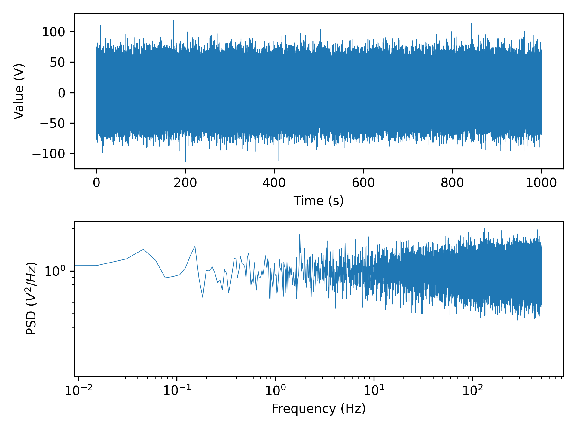
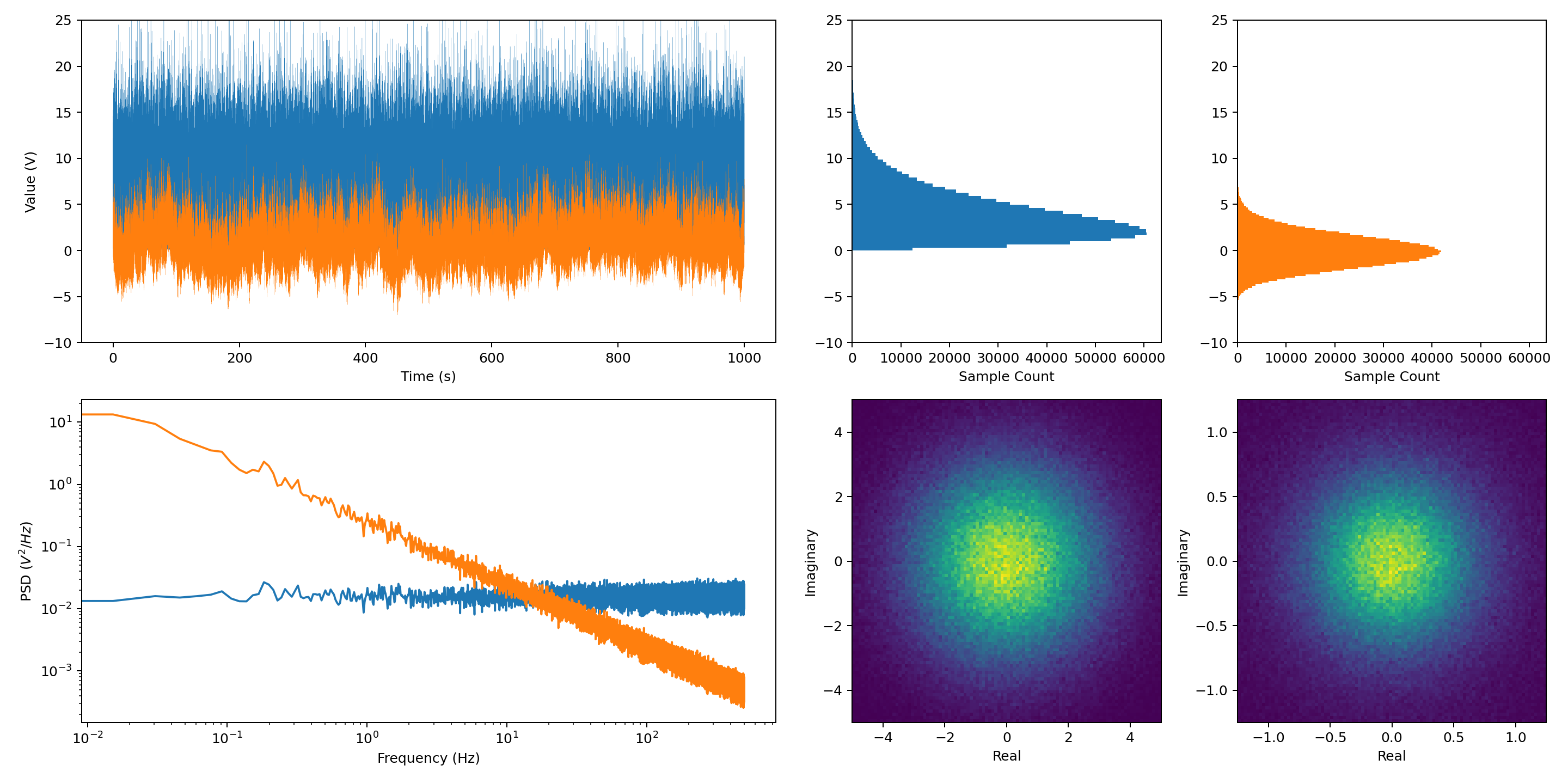
Judging from the plot above, we do indeed have a white noise signal with a PSD close to 1.0 over most of the frequency band.

Those that looked at the implementation of NoiseGenerator closely would’ve noticed the inefficiency of generating random noise in the time domain, then transforming it to the frequency domain, then transforming it back into the time domain. It’s possible to generate the white noise directly in the frequency domain². Here’s an alternative implementation of _base_noise() that does exactly that.

    def _base_noise(self, dt, n):
        # Calculate random frequency components
        f = np.fft.rfftfreq(n, dt)
        x_f = self.rng.normal(0,
            0.5, len(f)) + 1j * self.rng.normal(0, 0.5, len(f))
        x_f *= np.sqrt(n / dt)

        # Ensure our 0 Hz and Nyquist components are purely real
        x_f[0] = np.abs(x_f[0])
        if len(f) % 2 == 0:
            x_f[-1] = np.abs(x_f[-1])
        
        return f, x_f

Shaping the Spectrum

At this point, all that is left is to colour the noise by shaping its spectrum. Updating generate() to handle a colouring function is a suitably generic way to do this. We’ll add some helper static functions to the class for common colours, but of course you’re welcome to do something completely custom. There are really only two things to note here:

1. The PSD is directly proportional to the square of the FFT, so we need to take the square root of our colouring functions.
2. A few noise colours have $f$ in the denominator of a fraction, so we need to specifically handle the case that $f = 0$.

    def generate(self, dt, n, colour=None):
        f, x_f = self._base_noise(dt, n)

        if colour:
            x_f *= np.sqrt(colour(f))

        return np.fft.irfft(x_f)
    
    @staticmethod
    def pink(scale=1.0):
        """Creates a pink noise colouring function.

        Parameters
        ----------
        scale : float, optional
            Multiplier to adjust the scale of the pink noise.
        
        Returns
        -------
        function
            Pink noise colouring function that can be used with `generate()`.
            The function returned will be :math:`y(f) = s / f`, where :math:`s`
            is `scale`. At f = 0, the function will simply return 0.0.
        """

        return lambda f: scale / np.where(f == 0.0, np.inf, f)

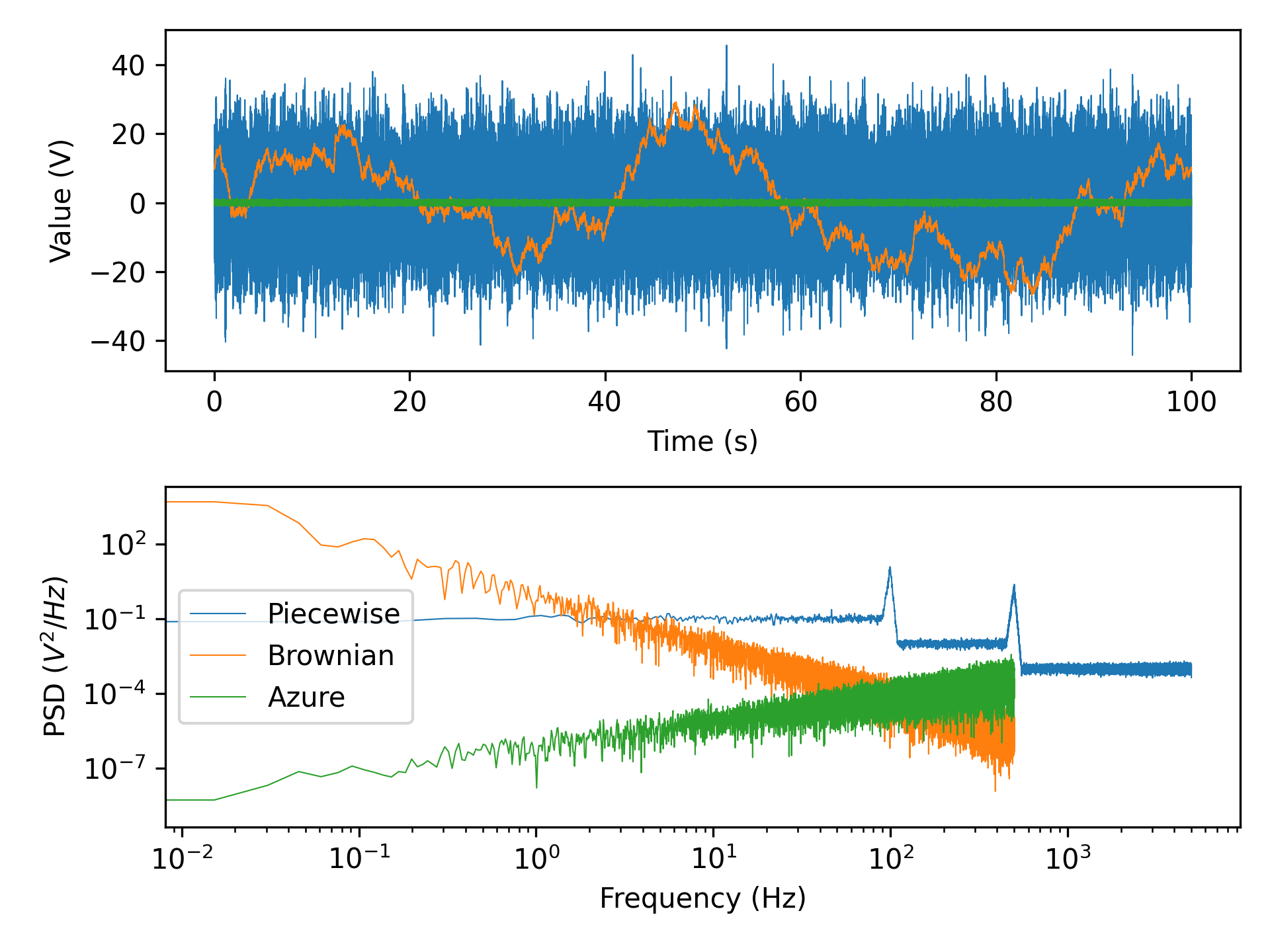
I’ve omitted most of the colours in the code snippet above, but the full NoiseGenerator class can be found in this gist. Of particular interest is the piecewise colouring function, which allows creation of some funky noise that can’t be classified by any of the standard colours.

ng = NoiseGenerator()
noise_settings = {
    "Piecewise": {
        "dt": 1e-4,
        "n": 1000000,
        "colour": ng.piecewise_logarithmic(
            [90.0, 100.0, 110.0, 450.0, 500.0, 550.0],
            [0.1, 10.0, 0.01, 0.01, 2.0, 0.001]
        )
    },
    "Brownian": {"dt": 1e-3, "n": 100000, "colour": ng.brownian()},
    "Azure": {"dt": 1e-3, "n": 100000, "colour": ng.azure(1.0e-6)}
}
for name, settings in noise_settings.items():
    x_t = ng.generate(**settings)
    plot_psd(x_t, settings["dt"], nperseg=65536)
plt.legend(noise_settings.keys())

Questions Raised

Although the coloured noise generation class worked perfectly for my needs, a few questions were raised while I was using it. I’ve left them unanswered for the moment, but if anyone has any answers, please get in touch.

Noise Distribution

The probability density function used in the random number generation above is Gaussian. It’s important to note that the noise distribution is a separate concept entirely to its power spectral density. For our base noise generation in the time domain, we could have used a uniform distribution, or an exponential distribution, or a gamma distribution, and they all would’ve worked.

Interestingly, after taking a Fourier transform, all of these distributions produce something that looks roughly like a 2D Gaussian distribution in the complex plane. Furthermore, after shaping the PSD using a colouring function and taking an inverse Fourier transform, we always seem to end up with noise in the time domain that tends towards a Gaussian distribution.

1. Is it possible to generate noise with a specific distribution in the frequency domain?
2. Why does shaping noise in the frequency domain tend to shift the time domain distribution towards a Gaussian distribution? Is it something to do with the central limit theorem?
3. Is it possible to generate noise with both a specific distribution and a specific colour that isn’t white?

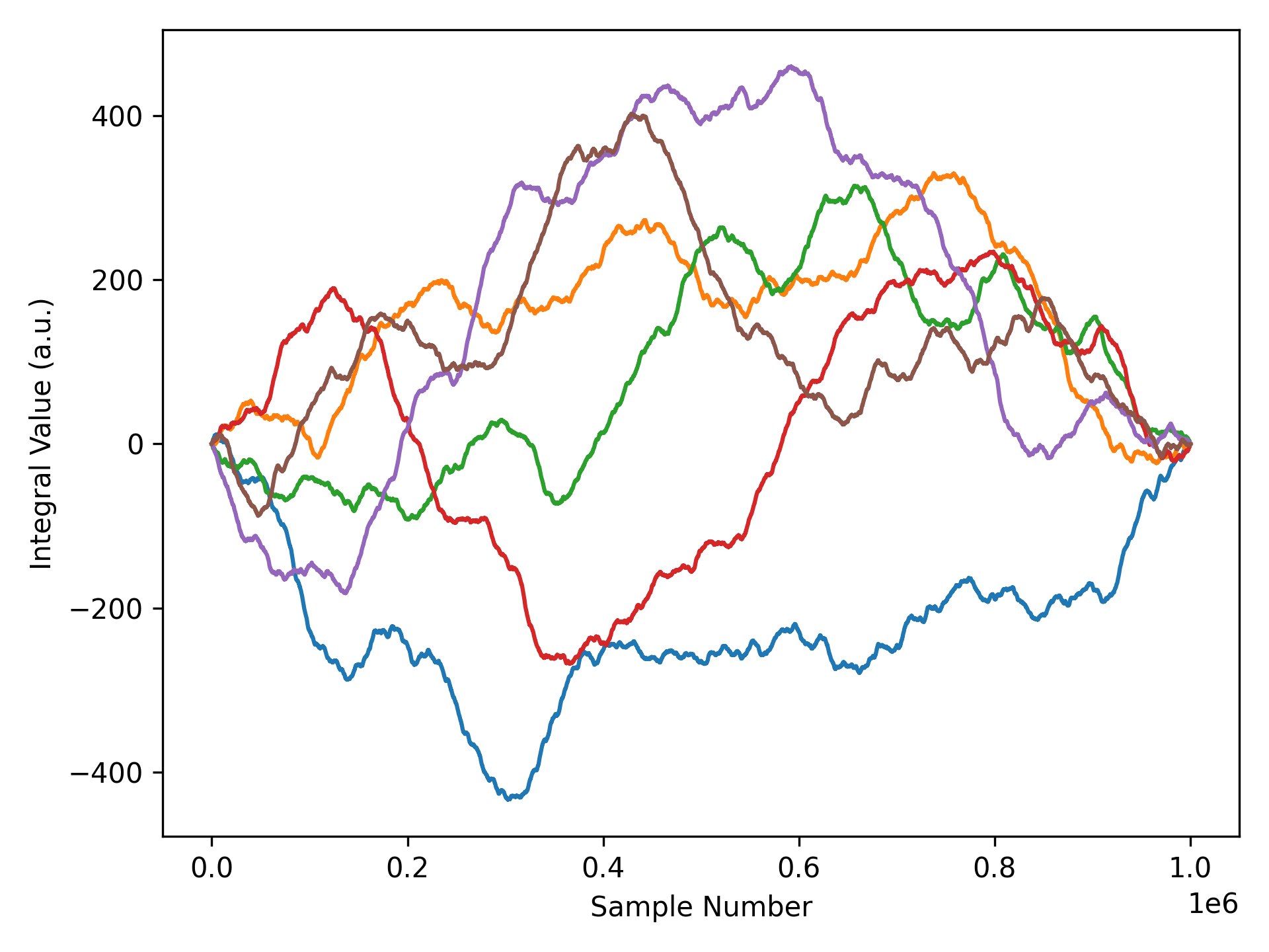
Integration of Noise

I was using the synthetically generated noise to simulate a gyroscope, so I’d integrate the signal to calculate the angular error of the system. In this way, I could test out bias estimation and compensation algorithms without having to acquire long datasets from a real gyroscope. I noticed some strange behaviour in the integrated signal, though. For all coloured noise that had a 0 Hz frequency component of 0.0, the resulting integral would have both a start and end value of 0.0. This of course meant that if I generated 1 million noise samples, my angular error at the millionth sample would always be 0.0.

What is going on here? My current theory is that it is due to the definition of the discrete Fourier transform:

$$X_k = \sum_{n=0}^{N-1} x_n \cdot e^{-\frac {i 2\pi}{N}kn}$$

If the Fourier transform is 0.0 for $k=0$, the above simplifies to:

$$0.0 = \sum_{n=0}^{N-1} x_n$$

Of course, this is exactly the oddity that we see - the sum of our noise samples is 0.0. It does raise the question of whether setting the 0 Hz component in our colour shaping functions to 0.0 is sensible. Perhaps it should be some other value?

Final Words

This small dive into noise generation techniques resulted in a NoiseGenerator class that was useful for gyroscope simulations, as well as other applications. At just 44 lines of functional code, it is testament to the power of the scientific computing libraries in the Python ecosystem. Although generating white noise and filtering it seems to be an accepted technique for coloured noise generation, it did raise some questions on the structure of the generated noise which I hope will be answered in the future.