
Haptick, Part Two
Bring-up and testing of a prototype 6DOF input device
As explained in Part One, I’m attempting to build a tactile input device using a force sensor with six degrees of freedom. At the end of the previous chapter, I was waiting on prototype parts to test a proof of concept device based on a Stewart platform with six force sensors integrated into the printed circuit assembly itself.
Well, the parts arrived, and thus began the first prototype iteration — assemble, test, learn and improve.
Remember, the goal of this prototype was to see if it was possible to:
- Take force measurements of each arm of a Stewart platform and calculate the torques and forces applied to the platform.
- Integrate load cells directly on the printed circuit boards themselves.
- Use thick-film resistors as strain gauges.
- Emulate the universal joints in the Stewart platform by making the trusses out of a bendable material (copper).
Construction
The general construction of the prototype was fairly straightforward. I spent some time populating the PCBs by hand, but it went very smoothly thanks to the limited number of different components and the interactive bill of materials generated by the excellent KiCad InteractiveHtmlBom plugin. Everything was hand soldered with a soldering iron except the tiny 0.4mm pitch QFN-32 package, for which I used hot air.
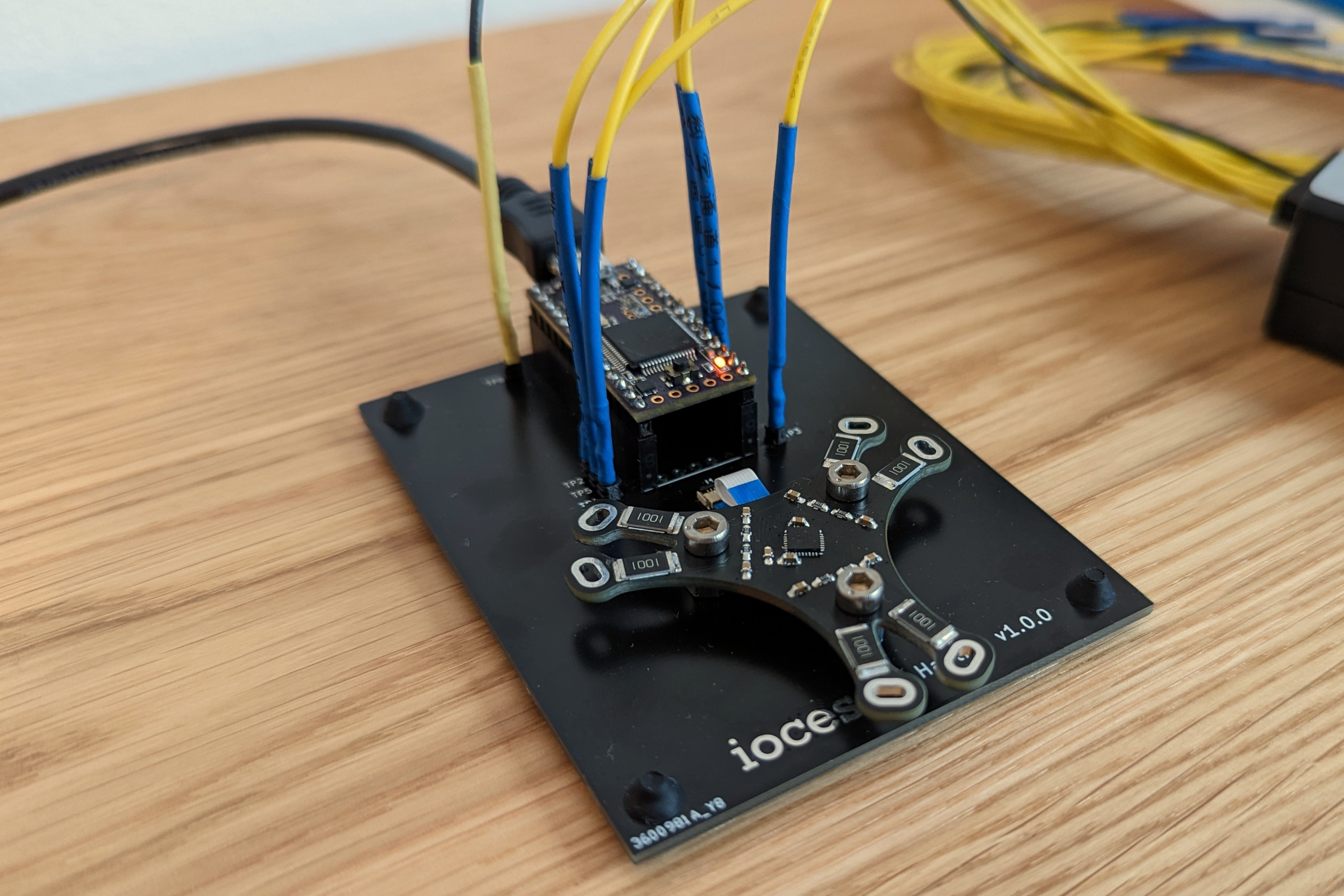
I split the mechanical assembly into two. Initially I only mounted the base of the Stewart platform to the interface board so I could do the board bring-up with access to the bulk of the circuitry and the individual load cells. I started on the test firmware with the same partial assembly and only mounted the platform in place once I was happy with the performance of the electronics.
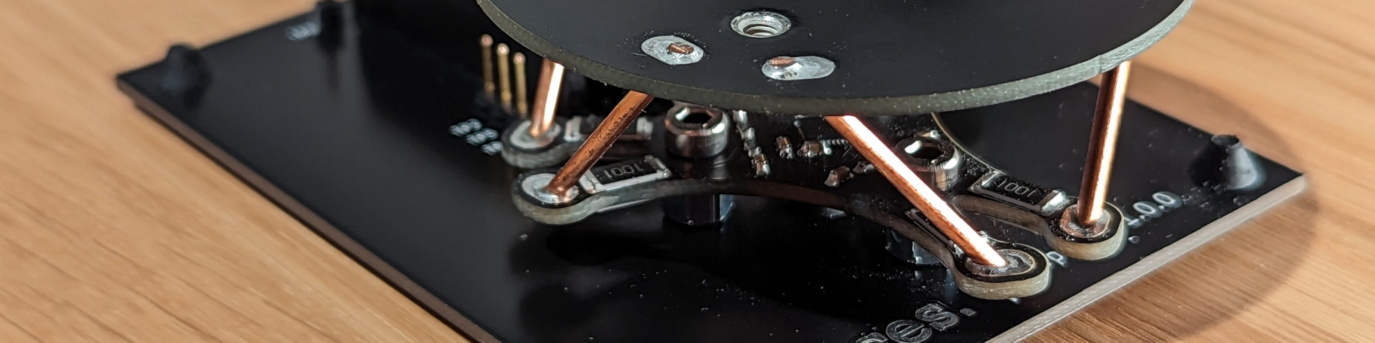
Mounting the platform started with stripping and straightening short sections of 2.5 mm² solid-core wire. After inserting each section through the slots in both the base and platform, I fine tuned their lengths with side cutters. The platform felt pretty rigid once all of the trusses were inserted and fully engaged the edges of the slots. The final step was soldering each truss in place and trimming the excess copper.
Code
To test the prototype, I churned out two fairly minimal, but useful pieces of code. I’ve gotten the project to the point where I’m comfortable releasing it as open source, so if you’re interested in the hardware, firmware and software, check out the GitHub repository.
Firmware
The first chunk of code was the firmware running on the Teensy 3.2 development board. It generates an 8 MHz ADC clock, configures the ADC sample rates and channel gains and sets up a virtual serial port and some interrupts to be able to stream data. From there, its sole job is to pump the six channels worth of samples out to the attached computer at a rate of around 4 kSPS.
I considered implementing more functionality in the firmware, including filtering and calculation of torques/forces, but it wasn’t worth the effort of dealing with the constraints of the Arduino IDE and the hardware it was running on. Instead I did the bulk of the heavy lifting on the PC side in a custom test application.
Test Application
Custom debug and test applications are invaluable when developing electronics. The ability to visualise data live and implement processing algorithms in a high level language meant I could rapidly iterate and solve problems with the sensor.
During testing, I coded up an application that allowed me to:
- Plot time-series data from the ADC.
- Visualise power spectral density and RMS value of the signals.
- Control a virtual 3D cube using the forces and torques applied to the platform.
- Implement some basic signal processing including low pass filtering and bias correction.
I wrote the application in Python using Qt 6 and PySide6 for the UI toolkit, Matplotlib for plotting and ModernGL for 3D rendering. On the backend, pySerial was used for the serial communication with NumPy and SciPy handling most of the signal processing.
Results
I’ve jumped right into the results section here, as there was no real testing regime for this prototype. This “follow your nose” discovery-style testing works well in the early stages of a project when you’re just trying to prove a concept. As such, this section meanders around a bit, documenting the results and problems I faced along the way.
First Signal
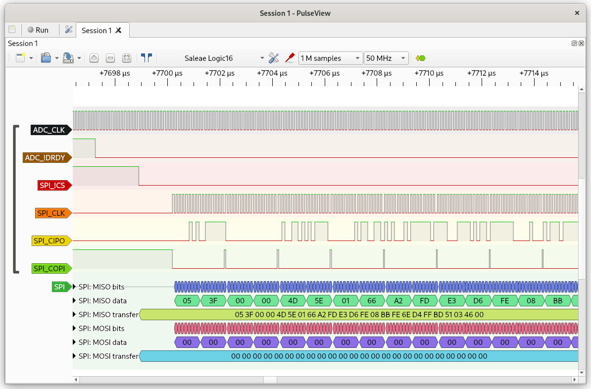
Interfacing with the ADS131M06 analog-to-digital converter was the first order of business. For the most part, the chip was already configured as I wanted it, and the slight tweaks I needed were just a few register settings away. The remainder of the interface was mostly timing and byte wrangling — handling interrupts and reading data from result registers into a local buffer. First data was probed and decoded using a USB logic analyser and PulseView from the sigrok project.
The rest of the firmware dealt with pulling data from the local buffers on the Teensy and streaming it out the virtual serial port. On the PC side, the test application read the data from the serial port, split the byte stream into samples and converted the 24-bit values back into voltages. The very first sample from each channel was assumed to be the offset for that channel.
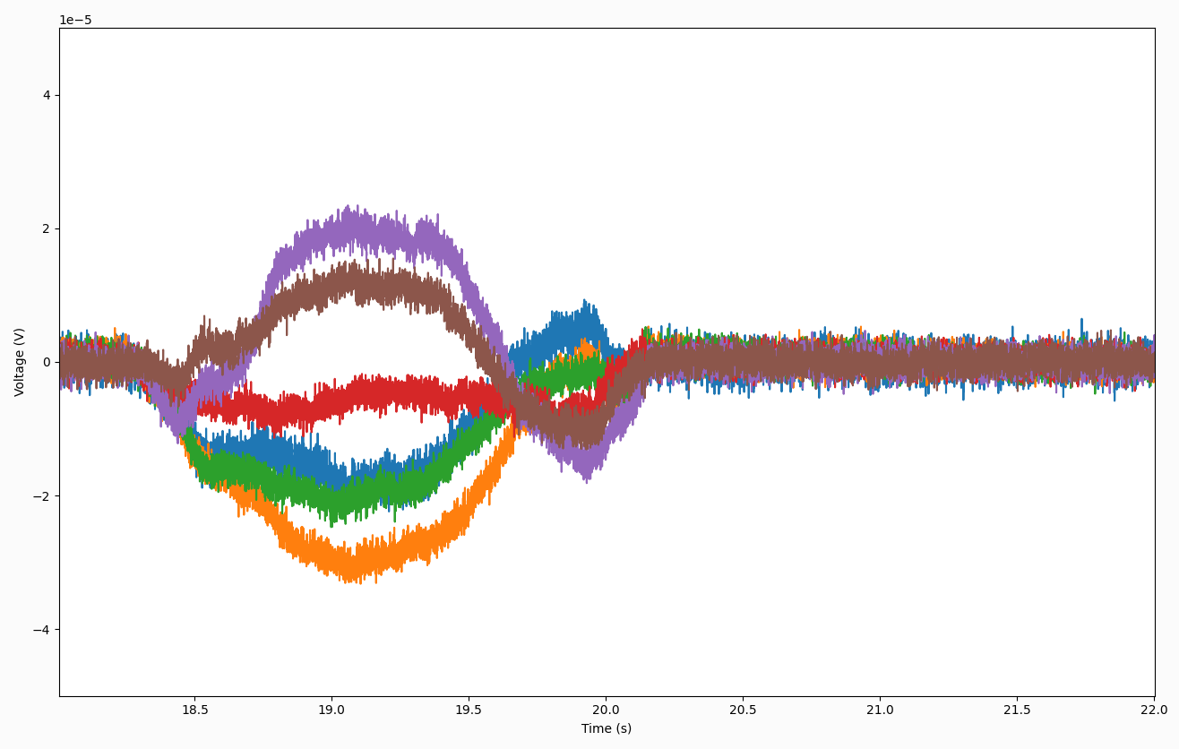
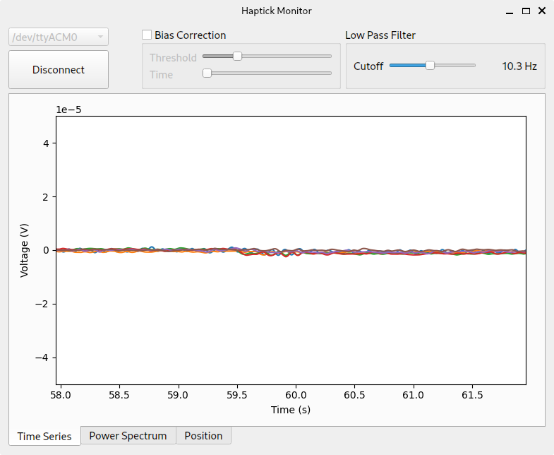
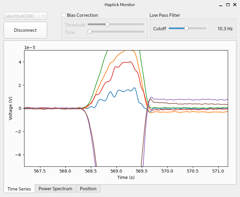
Initially the test application had no GUI, and the offset compensated data was just printed to stdout. This was the cusp of my black triangle moment, so I started pressing down on the arms of the Stewart platform base. Success! I could visibly see changes in values by lightly touching each arm.
Unfortunately, the digits were flickering so rapidly on the screen, it was hard to determine any sort of sensitivity of the load cells. I focussed my efforts on live plotting the data in the test application, and could soon see why. The signal was pretty noisy.
Dealing with Noise
I should preface this section by pointing out that there is very little filtering in the system. I put a token RC antialiasing filter in front of the ADC, and the ADC itself contains a sinc³ filter typical of delta-sigma converters. Ultimately, though, I’m sampling the load cells at 4 kSps and the bandwidth of the system is pretty close to the full 2 kHz Nyquist limit.
The ADS131M06 datasheet provides a nice performance table which indicates it should be contributing around 1.20 μV RMS of noise to the readings. Interestingly, running the preamplifiers at gains higher than 32 offers no benefits, and using higher oversampling rates achieves much the same noise reduction as a standard averaging filter ($1/\sqrt{N}$, where $N$ is the number of averaged samples). This indicates to me that the noise is likely dominated by input noise of the preamplifiers.
To quantify the noise levels of the prototype, I updated the test application to calculate and plot live power spectral density and display RMS values from the last second of data. The resulting noise levels were close to those specified in the ADC datasheet, with the exception of channel 1. I don’t have any concrete explanation for the higher noise of channel 1, but it could be due to PCB layout or assembly issues. I had to reflow the fine pitch QFN package a couple of times, and I’m still not 100% happy with the solder job.
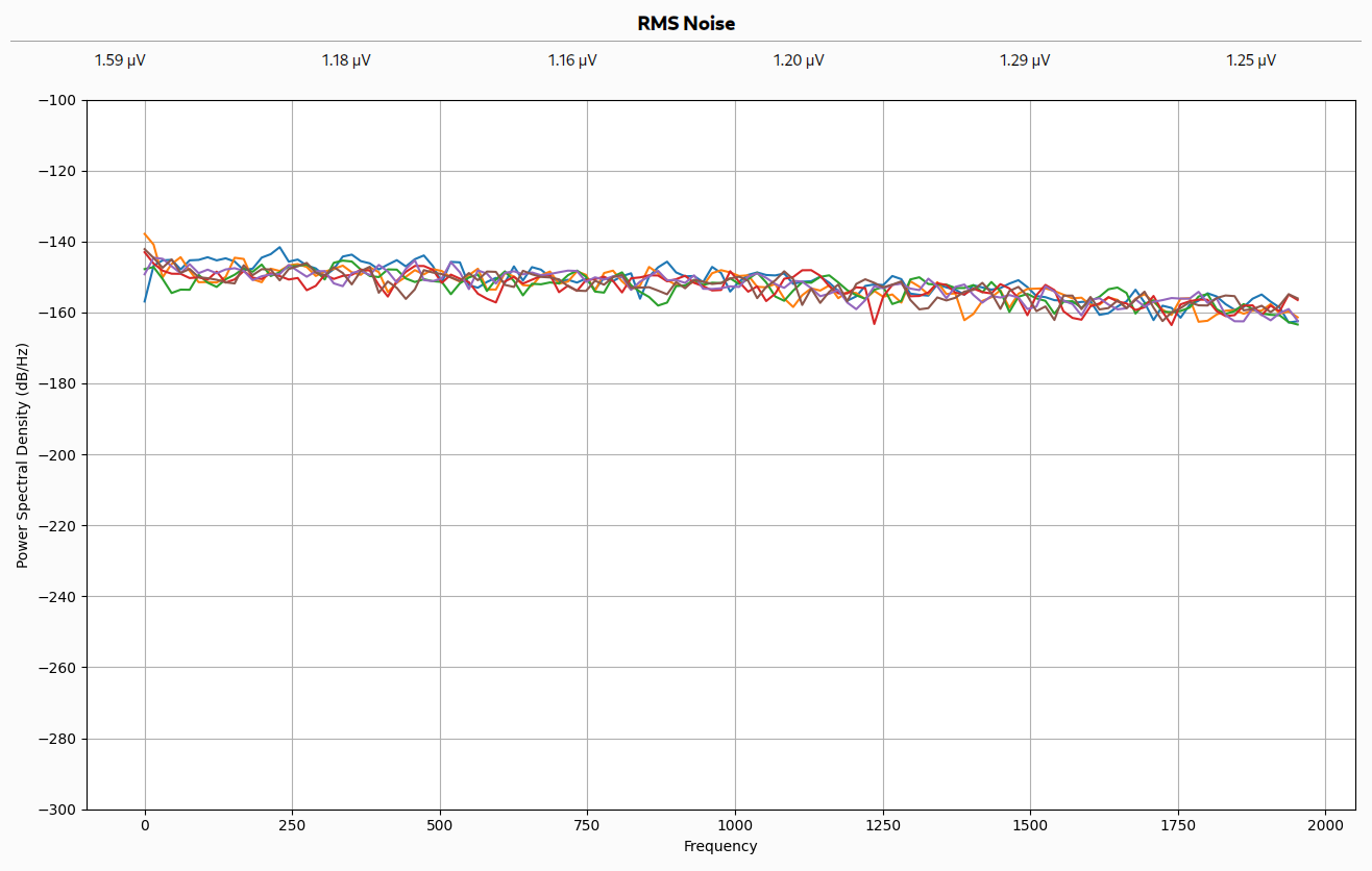
The noise was consistent across the bandwidth of the device, with a very minor rolloff at higher frequencies. This was good news as it meant I could significantly reduce the noise with a low pass filter. The big question is, where should I put the cutoff frequency?
In the age of 8 kHz mouse polling for extreme gaming, one might be excused for believing that humans have super quick reaction times and can move at high frequencies. The reality is that human reaction times average around 250 ms for visual stimulus, and even high performers rarely have reaction times faster than 100 ms. In regards to movement frequency, I don’t think humans can produce audible frequency oscillations with their hand or arm muscles, which would put their bandwidth down in the tens of hertz.
I updated the test application and implemented a 4th order Butterworth filter with a user configurable cutoff frequency. The power spectrum plot and noise level calculations confirmed its effectiveness, and allowed me to find a compromise between noise level and responsiveness of the sensor.
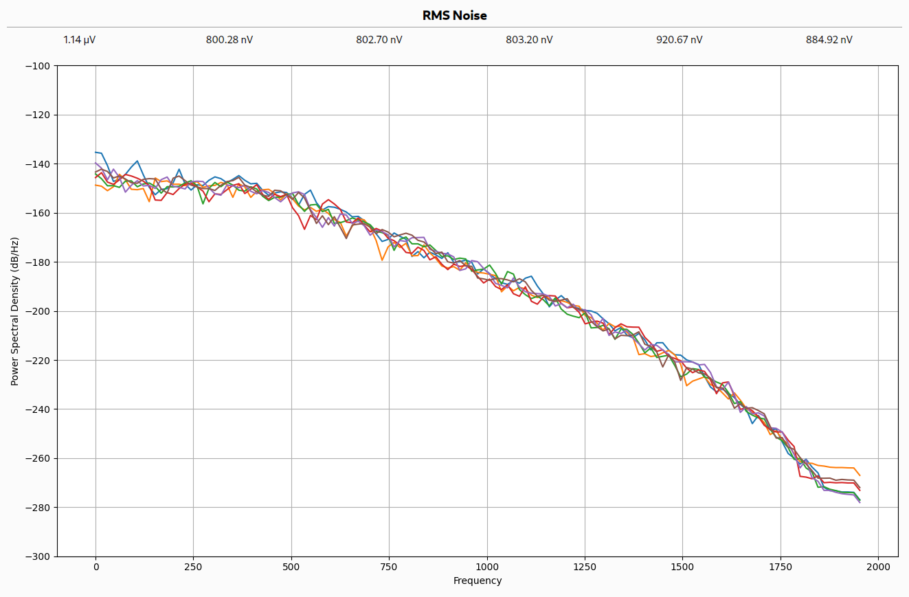
To me, the device still felt responsive even with the cutoff as low as 10 Hz. With that cutoff frequency, the RMS noise levels were reduced down to approximately 200 nV.
Ergonomics
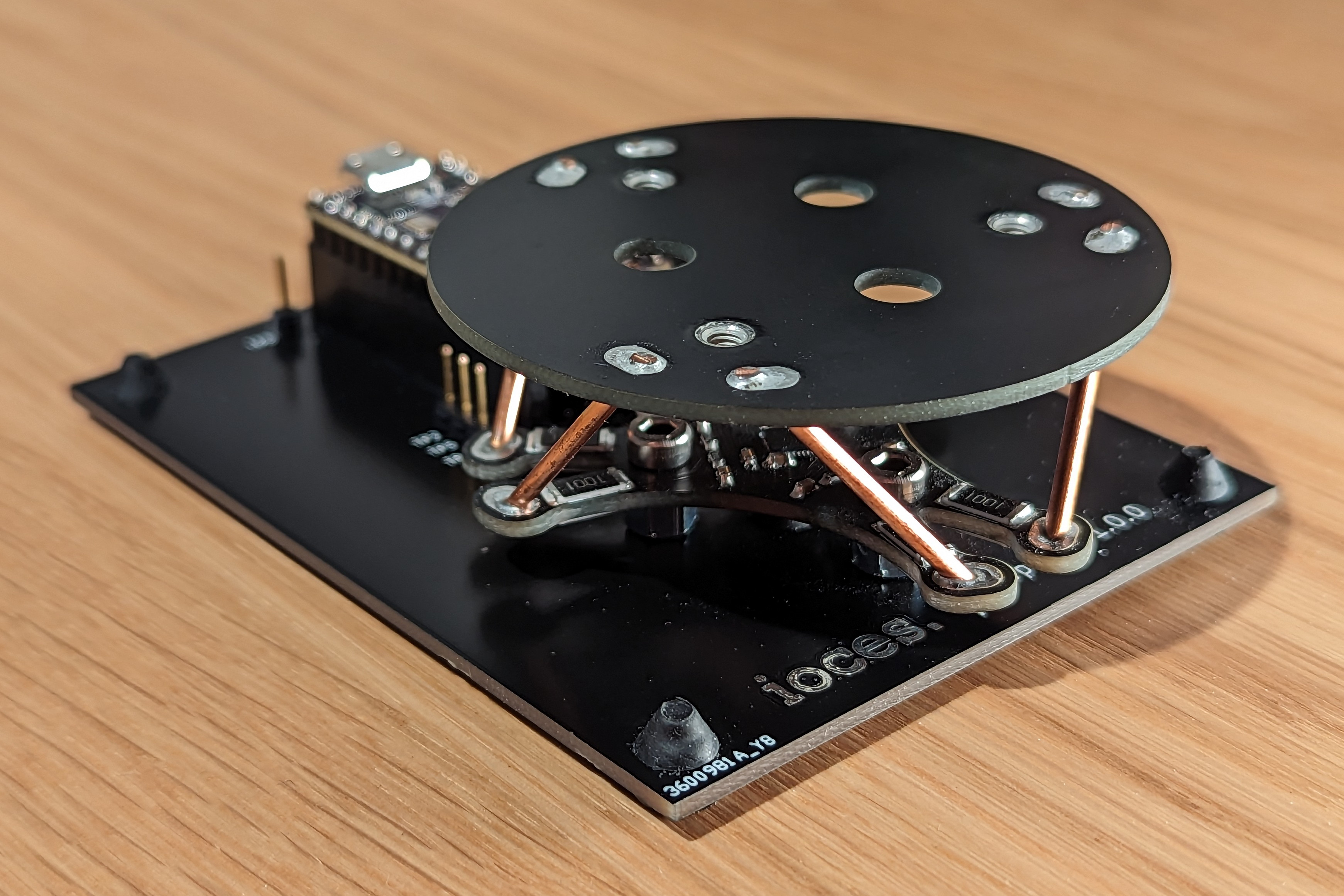
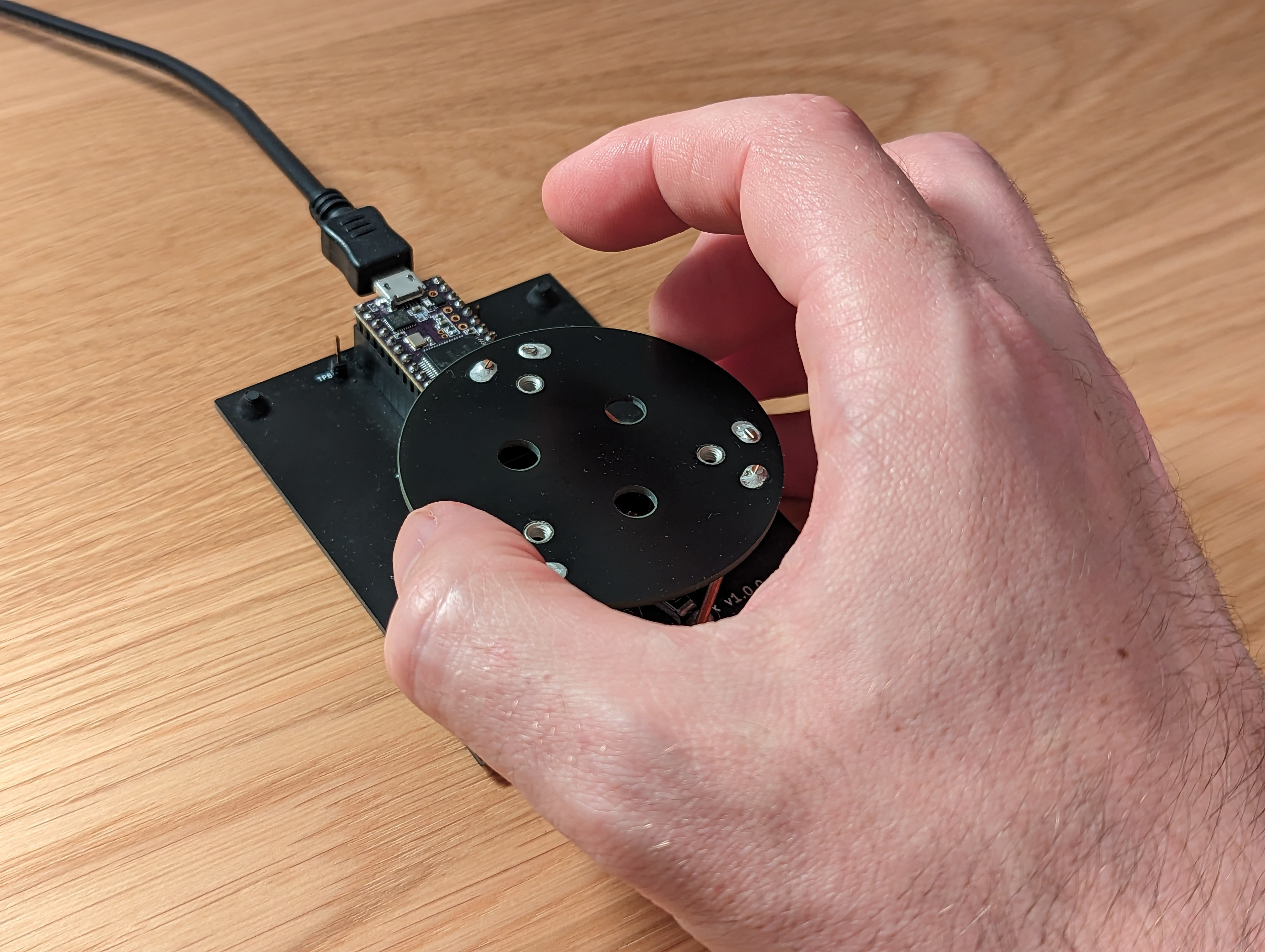
At this point I wanted to get an idea of the scale of the measurements to hand applied inputs, so I finished the assembly by soldering the trusses and platform into place. Although ergonomics weren’t really the focus of this initial proof of concept, I immediately made some observations when I started to apply forces and torques to the platform with my hand:
- The weight of the base/interface boards and rubber feet aren’t sufficient to hold the device in place.
- A disc isn’t a very pleasant shape to manipulate.
- The diameter of the platform is roughly correct for my sized hands, but the platform is positioned slightly too low.
- Access to the back of the platform by my fingers is limited due to the position and proximity of the Teensy board.
These should be easy to improve upon for future prototypes by:
- Using a much heavier, grippier base or switching to a design using suction caps.
- Installing a knob over the top of the platform that provides a better geometry to hold.

Sensitivity
With the platform installed I could easily test the sensitivity in real world units. I spooled up the test application, allowed it to calculate a baseline and then placed a known mass onto the platform. A 390 g mass placed in the center resulted in a response of 5 µV for each of the 6 channels. By my calculations, this results in a sensitivity of 7.8 µV/N.
That’s not great. Light touches to move a mouse are somewhere in the order of 200–300 mN, and a button click is ≈500 mN. For Haptick, those forces are distributed across 6 channels, so we need to be able to nicely sense forces with magnitudes down in the range of 40-50 mN. These sorts of forces will result in a response of ≈350 nV, which is barely out of the noise.
In short, while the SMD thick-film resistors are surprisingly sensitive to strain, they’re not sufficient for this application. For now, I’ll just apply higher forces and torques to this prototype, but in the long run the design will have to move to proper strain gauges. My very rough calculations indicate that strain gauges should be roughly two orders of magnitude more sensitive.
Inversion and Responsiveness
The mathematics behind finding the inverse function that converts measured truss forces back into forces and torques applied to the platform was covered in Part One. One of the concerns with this prototype was that the lack of universal joints would render this inverse function non-applicable. Doing the static analysis for the system without those joints looked like a nightmarish task.
I used soft copper wire for the trusses in the hope that it would flex around the joints and partially emulate a universal joint, but the approximation still needed to be proven. Without the facilities to apply precise torques and forces in all directions to the platform, I decided instead to jump to a full end-to-end test. If I could nicely control a model in 3D space by pushing, pulling and twisting the platform, it didn’t really matter if the inversion wasn’t perfect.
Adding that functionality to the test application took me down a long, winding path. The plan was to render a 3D cube in space and rotate/translate it using the prototype Haptick. Rather than pull in a big dependency like ursina, I figured I’d do it using the lower level ModernGL OpenGL bindings. That proved to be a bad decision. I ended up buried in GLSL shader code, texture mapping, OBJ file reading and homogeneous coordinates. After much yak shaving, I got to where I wanted.
The video above demonstrates the prototype in action. The cube’s linear velocity is controlled by the applied force calculated by the inverse function, and the rotation velocity is set by the applied torque. By adjusting some sensitivity coefficients, I switch between three different modes — controlling rotation only, controlling translation only and controlling both simultaneously.
It’s difficult to convey via video, but the device feels surprisingly snappy and intuitive. There are two major problems, however - crosstalk and drift.
Crosstalk
When controlling both the rotation and translation simultaneously, there is obvious crosstalk between the two. Pushing the platform to the right ($+x$ direction) also causes a roll about the $+y$ axis. The cause of this is almost certainly due to the lack of universal joints. The soft copper wire simply doesn’t approximate a universal joint sufficiently.
To solve the problem, I first considered trying to find an analytical solution to the static analysis of a universal-joint-less Stewart platform, something a commenter suggested on my LinkedIn post. I preempted the rabbit hole that would lead me down, so instead considered dumping it into a FEA package like SimScale.
At some point during this thought process, I realised I was attempting to simulate a system I’d already physically built. Why couldn’t I just measure the response to three orthogonal force vectors and three orthogonal torque vectors and use them to find the inverse function? The math ends up pretty simple if we assume the system is linear.
$$ \begin{bmatrix} a_{11} & a_{12} & a_{13} & a_{14} & a_{15} & a_{16} \\ a_{21} & a_{22} & a_{23} & a_{24} & a_{25} & a_{26} \\ a_{31} & a_{32} & a_{33} & a_{34} & a_{35} & a_{36} \\ a_{41} & a_{42} & a_{43} & a_{44} & a_{45} & a_{46} \\ a_{51} & a_{52} & a_{53} & a_{54} & a_{55} & a_{56} \\ a_{61} & a_{62} & a_{63} & a_{64} & a_{65} & a_{66} \\ \end{bmatrix} \begin{bmatrix} \lang\bm{F}_1\rang_z \\ \lang\bm{F}_2\rang_z \\ \lang\bm{F}_3\rang_z \\ \lang\bm{F}_4\rang_z \\ \lang\bm{F}_5\rang_z \\ \lang\bm{F}_6\rang_z \end{bmatrix} = \begin{bmatrix} \lang\bm{F}_p\rang_x \\ \lang\bm{F}_p\rang_y \\ \lang\bm{F}_p\rang_z \\ \lang\bm{M}_p\rang_x \\ \lang\bm{M}_p\rang_y \\ \lang\bm{M}_p\rang_z \end{bmatrix} $$In the equation above, $a_{mn}$ are calibration coefficients, $\bm{F}_p$ is the force applied to the platform, $\bm{M}_p$ is the torque applied to the platform and $\bm{F}_i$ is the force vector applied to the platform by the $i$th truss ($=F_i \hat{\bm{u}}_i$ from Part One). Component $j$ of vector $\bm{v}$ is denoted as $\lang \bm{v} \rang_j$.
To perform the calibration, six linearly independent forces and torques need to be applied to the platform while measuring the response. This will result in a system of 36 simultaneous equations which can be used to solve for the 36 calibration coefficients.
Measurement Drift
The second issue I discovered during the end-to-end test was measurement drift. Various things cause this, and I identified a few candidates during testing. Temperature changes caused ADC readings to shift, which was especially noticeable when the device was first powered on and began to warm up. Larger input forces and torques also seemed to cause plastic deformation in the Stewart platform. After a “robust” input, the ADC readings would not return to the same zero point as before that input.
This was anticipated, and my plan was to continually rezero the measurements when I detected the Haptick prototype was untouched. I wanted to use the truss force signals themselves to detect when a hand was touching the device. The assumption was that a person would never have a completely motionless hand when using the device and small tremors would be able to be used to detect touch.
I implemented a rolling standard deviation check that assesses whether the standard deviation of each truss force is below a particular threshold for a specified amount of time. When this check is asserted, readings are rezeroed based on the mean value of the signals over the same period of time.
Unfortunately, due to the very low signal-to-noise ratio of the system, small tremors are not detectable and the standard deviation threshold needs to be set quite high. Because of this, the bias correction algorithm regularly rezeros the signal while the device is being manipulated. This results in the user having to compensate and the cube drifting away when the platform is released.
I’d still like to see if I can solve the drift issue using just the truss force measurements themselves, but it will require a significantly more sensitive device. Failing that, I’ll attempt to use the knob as a capacitive touch sensing electrode to determine when it is being gripped.
The Next Prototype
As of the date of publishing, I’ve already begun to iterate on the design. New PCBs and components for the next prototype have been ordered and received. I still need to design and 3D print some parts, then begin assembly. That will kick off the next round of testing and a future blog post. The changes I’ve made are:
- Switching to strain gauges instead of using thick film resistors. I’ve purchased a pack of BF350-3AA strain gauges from a random seller on Aliexpress. I’ll attempt to surface mount solder the gauges onto the PCB using hot air, then underfill the active area with cyanoacrylate adhesive.
- Increasing the bridge source impedances to allow for lower filter cutoff frequencies. The existing design achieved noise performance on par with what was expected, but it doesn’t hurt to have the component footprints on the board to be able to tweak the antialiasing filtering a little more.
- 3D printing a knob to mount to the platform for something nicer to hold.
- Designing some fixtures that will allow for calibration of the device.
The problem of the device sliding across the desk won’t be solved in this next iteration, but hopefully the changes above will allow fixing of the measurement drift, crosstalk and slightly improve ergonomics.
Conclusion
Let’s briefly revisit the initial questions this prototype was supposed to answer. We now have enough information to provide some insights:
- A Stewart platform is a very promising way to implement a six degree of freedom force/torque sensor. Indeed, since Part One, there has been at least one other device using the same concept.
- The cantilever beams milled into the PCB geometry work great. FR4 PCB material may have some hysteresis issues, but it likely isn’t a problem for this application.
- Thick film resistors can effectively be used as strain gauges. If you want a cheap way to measure forces in the several hundred millinewton sort of range, they’d be a good option. Unfortunately, they aren’t sensitive enough for use in Haptick.
- The soft copper trusses don’t fully emulate universal joints, and there are still non-axial torques transmitted through them. A possible workaround is to account for these torques through a full calibration.
All in all, this was a satisfying first prototype that shows a lot of promise. The next iteration should iron out most of the remaining problems, and we can close out the proof of concept phase.